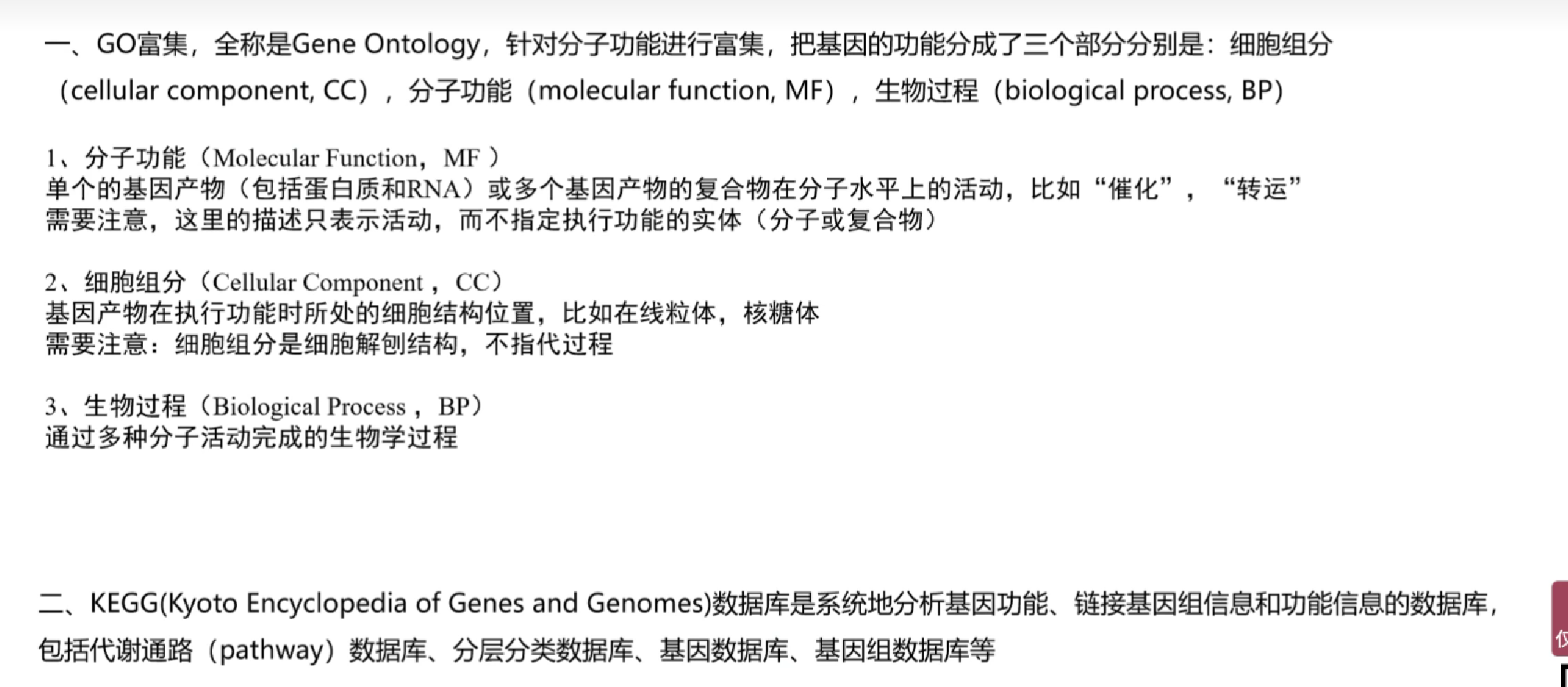
GO富集分析

富集分析函数★

基因列表、物种基因数据库、基因名称类型、是否将基因ID转换为基因名字

enrich.go <- enrichGO(gene = special_gene,  #待富集的基因列表
                      OrgDb = org.Hs.eg.db,  #指定物种的基因数据库，示例物种是绵羊（sheep）
                      keyType = 'SYMBOL',  #指定给定的基因名称类型，SYMBOL,ENSEMBL,ENTREZID三种类型
                      ont = 'ALL',  #GO Ontology，可选 BP、MF、CC，也可以指定 ALL 同时计算 3 者
                      pAdjustMethod = 'BH',  #指定用fdr作为 p 值校正方法
                      minGSSize = 10,  # 富集的GO条目至少包含10个基因，可以修改
                      pvalueCutoff = 0.05,  #指定 p 值阈值（<0.05）
                      qvalueCutoff = 0.2,  #指定 q 值阈值（<0.2）
                      readable = FALSE)   # 将GENE ID转为基因名字

go <- as.data.frame(enrich.go)
# 保存GO结果表
write.table(go, 'enrich.go.txt', sep = '\t', row.names = FALSE, quote = FALSE)

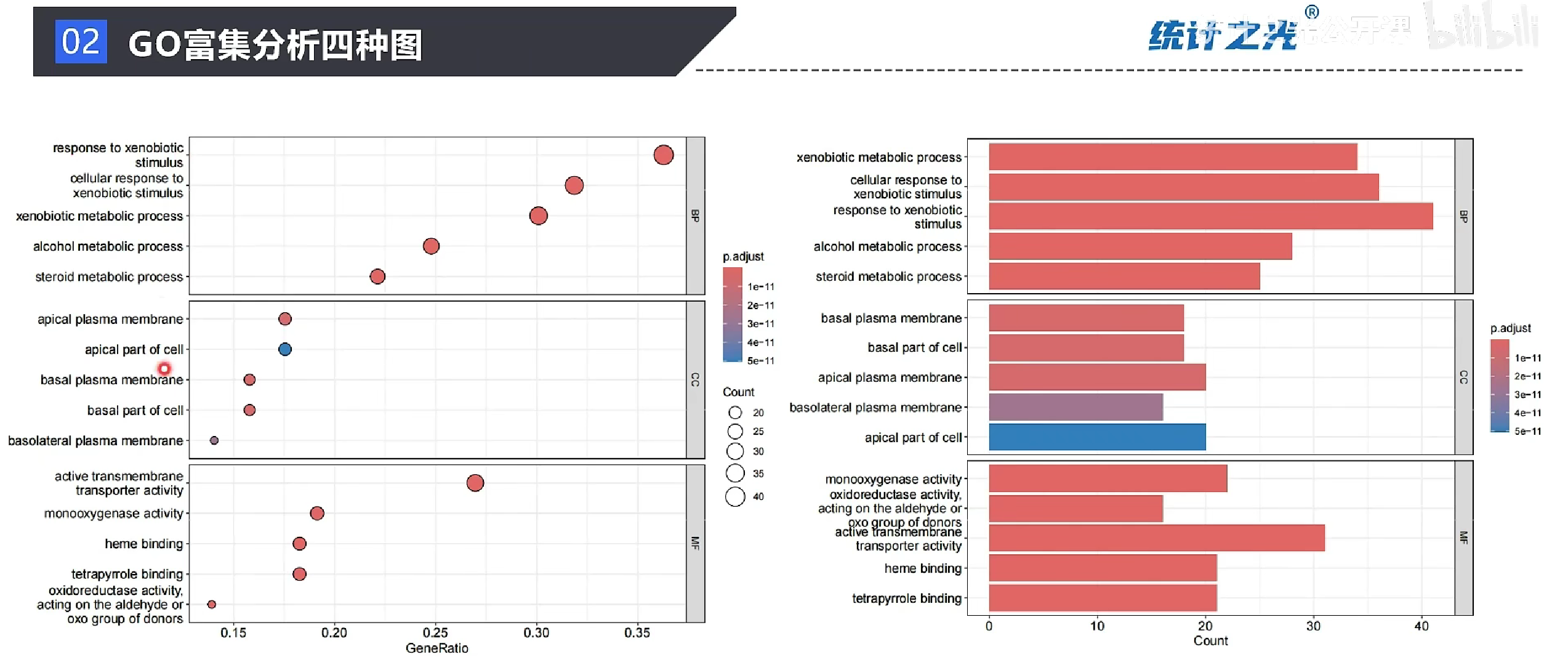
绘图

代码

library("ggplot2") 

pdf(file='GO_ALL_DOT.pdf',width = 10)
dotplot(enrich.go,split="ONTOLOGY",showCategory=5)+facet_grid(ONTOLOGY~.,scale="free")
## 用ontology来分框，每个框里面显示5个条目（前五个）
dev.off()

pdf(file='GO_ALL_BAR.pdf',width = 10)
barplot(enrich.go,split="ONTOLOGY",showCategory=5)+facet_grid(ONTOLOGY~.,scale="free")
## 用ontology来分框，每个框里面显示5个条目
dev.off()

library(dplyr)
#挑选BP，MF，CC的前5个term，按校正后的p值，升序排列

top5 <- enrich.go %>% group_by(ONTOLOGY) %>% top_n(n=-5, wt=p.adjust)
top_5 <- as.data.frame(top5)

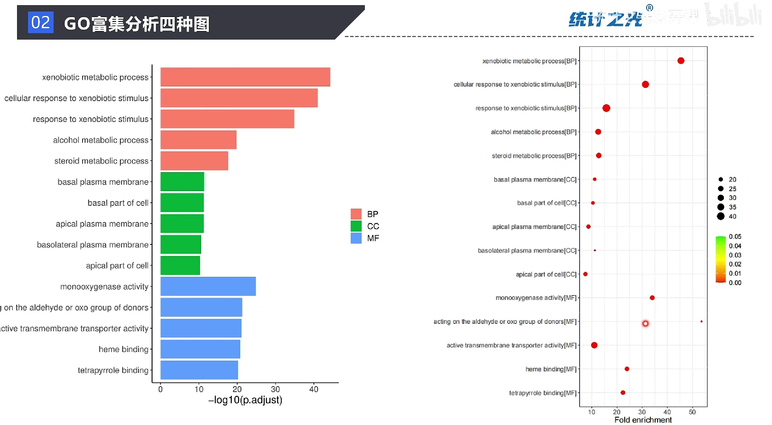
pdf("GO_barplot.pdf",width = 10)
#横轴是GO条目名字，纵轴是-log10(校正后的p值)，根据BP，CC类别填充颜色
ggplot(top_5,aes(x=Description,y=-log10(p.adjust),fill=ONTOLOGY))+
  geom_bar(stat="identity")+   #柱状图
  coord_flip()+  # 交换横轴与纵轴位置
  scale_x_discrete(limits=rev(top_5$Description))+  # 设置x轴上GO条目的顺序
  theme_classic()+  # 采用经典主题
  theme(
    text=element_text(size=15),  #所有的字体大小设置为20
    axis.title.y=element_blank(),  # y轴标签为空
    axis.title.x=element_text(size=15),  # x轴字体大小设为15
    legend.title = element_blank()   # 图标题为空
  )
dev.off()


#定义将geneRatio和bgRatio转换成小数的函数
f2d <- function(ratio){
  sapply(ratio,function(x) as.numeric(strsplit(x,"/")[[1]][1])/as.numeric(strsplit(x,"/")[[1]][2]))
}

#计算富集倍数，添加到go数据框最后一列
go_fe <- enrich.go %>% mutate(fe=f2d(GeneRatio)/f2d(BgRatio))
go_fe_df <- as.data.frame(go_fe)

#分别挑选BP，CC，MF的前5个term，按照校正后的p值，升序排列
top5_fe <- go_fe %>% group_by(ONTOLOGY) %>% top_n(n=-5, wt=p.adjust)

#每个GO条目后面加上对应的BP、CC或MF
top5_fe_term <- top5_fe %>% mutate(term=paste0(Description,"[",ONTOLOGY,"]"))

#转为数据框格式
top5_fe_term_df<-as.data.frame(top5_fe_term)

pdf("GO_ALL_DOT_inone.pdf",width = 10,height = 10)
ggplot(top5_fe_term_df,aes(x=term,y=fe,color=p.adjust,size=Count))+
  geom_point()+  ##散点图
  coord_flip()+  ## 交换x和y轴位置
  scale_colour_gradientn(limits=c(0,0.05),  #p值范围
                         colors = c("red","yellow","green"))+  #渐变颜色，p值越小，颜色越红
  scale_x_discrete(limits=rev(top5_fe_term_df$term))+  #设置x轴上GO条目顺序
  theme_bw()+  # 黑白主题
  ylab("Fold enrichment")+  #y轴标题
  theme(
    text=element_text(size=15),
    axis.title.y=element_blank(),
    axis.title.x=element_text(size = 15),
    legend.title = element_blank()
  )
dev.off()

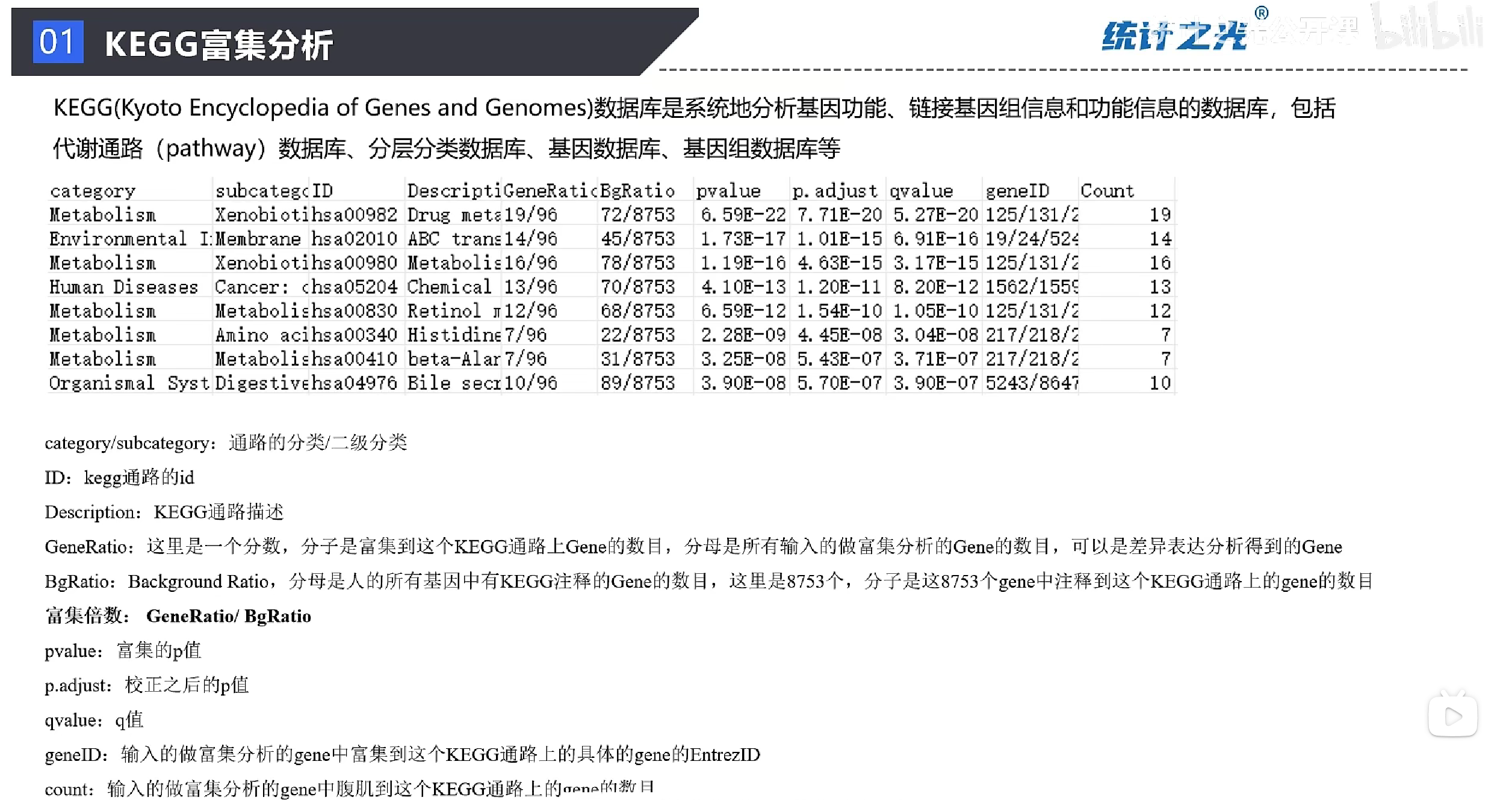
KEGG富集分析

分析函数

KEGG分析基因名称只能使用ENTREZID
此函数需联网查询

# 基因名称转换
entrezid_all = mapIds(x = org.Hs.eg.db,  #id转换的比对基因组（背景基因）的物种，以人为例
                      keys = special_gene, #将输入的gene_name列进行数据转换
                      keytype = "SYMBOL", #输入数据的类型
                      column = "ENTREZID")#输出数据的类型

enrich.kegg <- enrichKEGG(gene = entrezid_all,  # 这里需要输入的gene，ID只能未ENTREZID
                          organism = "hsa",  #富集物种为人，物种缩写可参考：https://www.genome.jp/kegg/catalog/org_list.html
                          pAdjustMethod = "BH", #指定用fdr作为 p 值校正方法
                          pvalueCutoff = 0.05,  #指定 p 值阈值（<0.05）
                          qvalueCutoff = 0.2)  #指定 q 值阈值（<0.2）
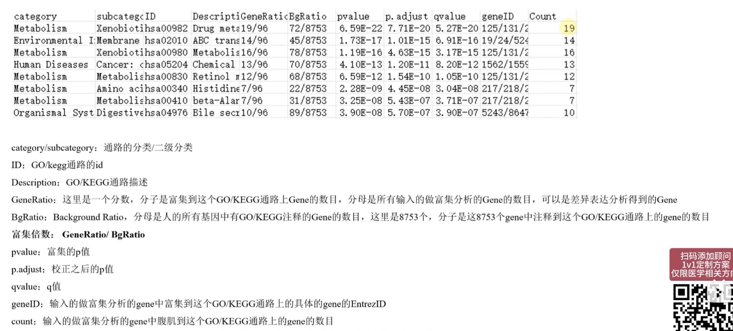
kegg_df <- as.data.frame(enrich.kegg)
write.csv(kegg_df,"kegg_enrich.csv",row.names = F)

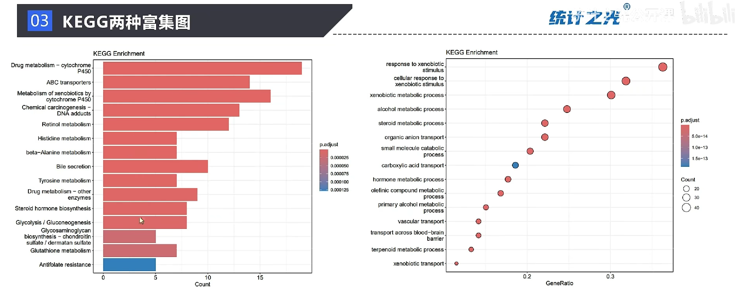
展示结果

pdf(file = "KEGG_bar.pdf",width = 10)
barplot(enrich.kegg,showCategory = 15,title = "KEGG Enrichment")
# 展示前15个
dev.off()

pdf(file = "KEGG_dot.pdf",width=10)
dotplot(enrich.kegg,showCategory=15,title="KEGG Enrichment")
dev.off()

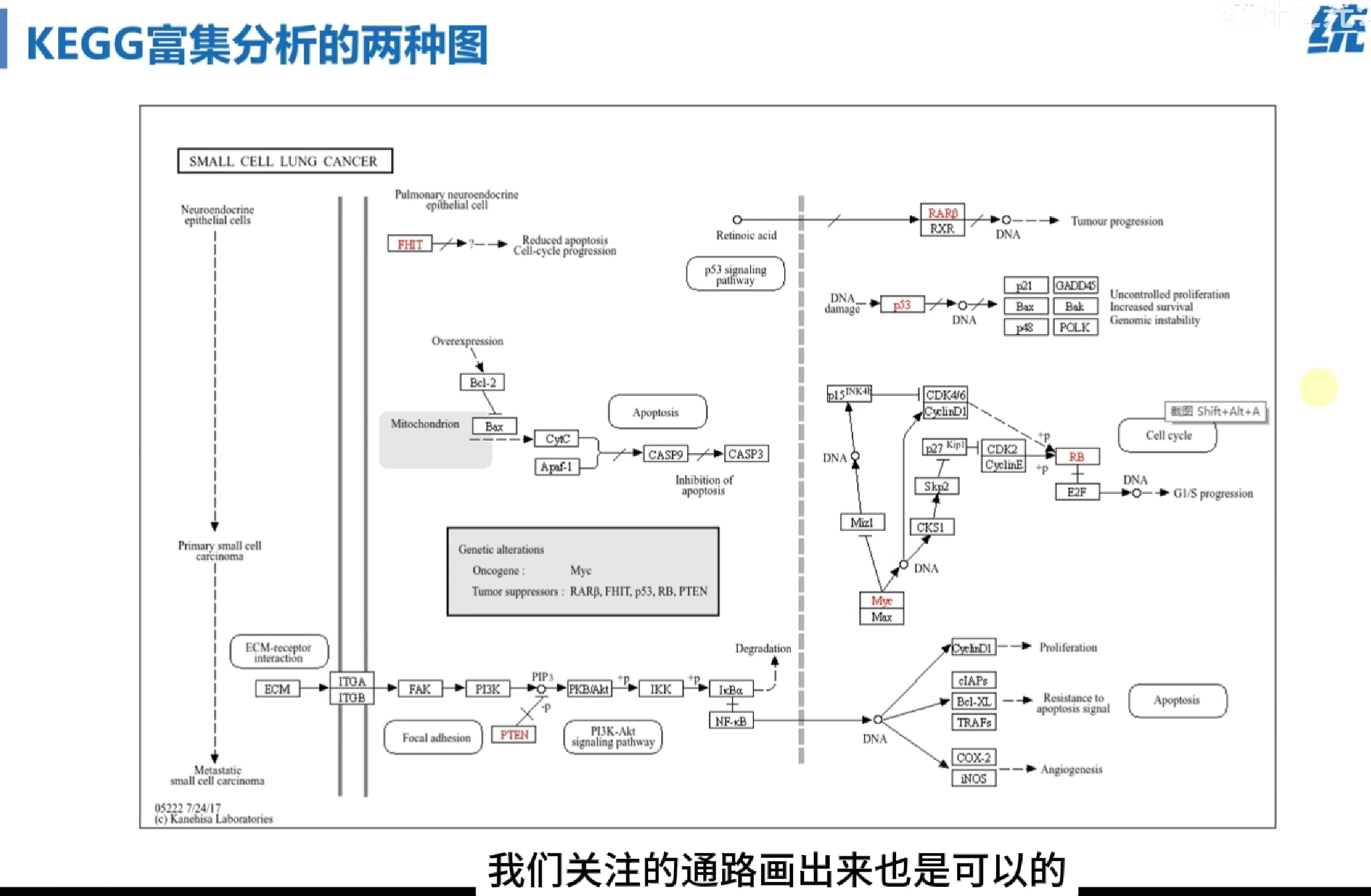
通路图

KEGG结果中的ID列——通路ID
绘图优点：标注出差异分析结果基因，及上下调水平
标注上下调水平需使用logFC

# BiocManager::install("pathview")
library(pathview)

# 2.3.1 简单版
## 以hsa00982通路举例，此处标记了所筛选基因
## 将所筛选基因列表、通路ID作为输入项
hsa00982 <- pathview(gene.data = special_gene,  #基因列表
                     pathway.id="hsa00982",   # 通路名
                     species ="hsa",   #物种
                     gene.idtype= "SYMBOL",   #基因id或名称类型，SYMBOL,ENSEMBL,ENTREZID  三种类型
                     kegg.native=TRUE)   #TRUE:输出png图片，FALSE：输出pdf文件


# 2.3.2 标注上下调水平版
## 此处还标记了所筛选基因的上下调水平
## 将行名为基因名，列名为logFC的数据、通路ID作为输入项
deg_kegg1 <- resSig[special_gene,]
deg_kegg2 <- deg_kegg1$log2FoldChange
view(deg_kegg2)
names(deg_kegg2) <- special_gene
hsa00982 <- pathview(gene.data = deg_kegg2,
                     pathway.id="hsa00982",
                     species ="hsa",
                     gene.idtype= "SYMBOL",  
                     kegg.native=TRUE,
                     limit=list(gene=max(abs(deg_kegg2)),cpd=1)
)

GO富集分析介绍

KEGG富集分析介绍